Custom derivative rules with hijax primitives

There have long been two ways to define differentiation rules in JAX:

1. using jax.custom_jvp and jax.custom_vjp to define custom differentiation rules for Python functions that are already JAX-transformable, as described in the custom derivatives notebook; and

2. defining new core.Primitive instances along with all their transformation rules, for example to call into functions from other systems like solvers, simulators, or general numerical computing systems.

Hijax primitives unify these two. A hijax primitive is a real JAX primitive: it appears as a single unit in jaxprs, and you can attach a rule for each transformation. But like a jax.custom_vjp-decorated function, it also carries a Python implementation, written in terms of ordinary JAX operations, which is used for evaluation and lowering. So you don’t need to write a lowering rule, and rules for the other transformations are only needed if you actually use those transformations.

This document shows how to use hijax primitives to define custom derivative rules for JAX-transformable Python code. It’s a hijax-flavored analogue of the custom derivatives notebook, and assumes familiarity with jax.jvp and jax.grad, and the mathematical meaning of JVPs and VJPs (see The Autodiff Cookbook).

Hijax is experimental: expect imports from jax.experimental.hijax, and expect the APIs to evolve. For stable APIs that cover most custom-derivative use cases, use jax.custom_jvp and jax.custom_vjp, described in Custom derivative rules for JAX-transformable Python functions.

TL;DR

Subclass VJPHiPrimitive, declare the input and output types, and define an expand method giving the implementation. Then attach the derivative rules you need: vjp_fwd/vjp_bwd_retval for reverse mode, jvp for forward mode:

import jax
import jax.numpy as jnp
from jax.experimental.hijax import VJPHiPrimitive

class SinTimesY(VJPHiPrimitive):
  def __init__(self, x_aval, y_aval):
    self.in_avals = (x_aval, y_aval)  # input types
    self.out_aval = x_aval            # output type
    self.params = {}                  # static parameters (none here)
    super().__init__()

  # Implementation, used for evaluation and lowering (e.g. under jit).
  def expand(self, x, y):
    return jnp.sin(x) * y

  # Reverse-mode: forward pass returns (primal_out, residuals).
  def vjp_fwd(self, nzs_in, x, y):
    return self(x, y), (jnp.cos(x), jnp.sin(x), y)

  # Reverse-mode: backward pass maps (residuals, output cotangent) to a tuple
  # of input cotangents.
  def vjp_bwd_retval(self, res, g):
    cos_x, sin_x, y = res
    return (cos_x * g * y, sin_x * g)

  # Forward-mode rule (optional, only needed under e.g. jax.jvp).
  def jvp(self, primals, tangents):
    (x, y), (x_dot, y_dot) = primals, tangents
    return self(x, y), jnp.cos(x) * x_dot * y + jnp.sin(x) * y_dot

def f(x, y):
  return SinTimesY(jax.typeof(x), jax.typeof(y))(x, y)

from jax import jvp, grad

print(f(2., 3.))
y, y_dot = jvp(f, (2., 3.), (1., 0.))
print(y)
print(y_dot)
print(grad(f)(2., 3.))

2.7278922
2.7278922
-1.2484405
-1.2484405

Note that, unlike with jax.custom_jvp and jax.custom_vjp where you must choose one or the other, a single hijax primitive can carry both forward- and reverse-mode rules.

Example problems

To get an idea of what problems hijax custom derivatives are meant to solve, let’s go over a few examples. A more thorough introduction to the VJPHiPrimitive API is in the next section.

Example: Numerical stability

One application of custom derivative rules is to improve the numerical stability of differentiation.

Say we want to write a function called log1pexp, which computes \(x \mapsto \log ( 1 + e^x )\). We can write that using jax.numpy:

def log1pexp(x):
  return jnp.log(1. + jnp.exp(x))

log1pexp(3.)

Array(3.0485873, dtype=float32, weak_type=True)

Since it’s written in terms of jax.numpy, it’s JAX-transformable:

from jax import jit, grad, vmap

print(jit(log1pexp)(3.))
print(jit(grad(log1pexp))(3.))
print(vmap(jit(grad(log1pexp)))(jnp.arange(3.)))

3.0485873
0.95257413
[0.5       0.7310586 0.8807971]

But there’s a numerical stability problem lurking here:

print(grad(log1pexp)(100.))

nan

That doesn’t seem right! After all, the derivative of \(x \mapsto \log (1 + e^x)\) is \(x \mapsto \frac{e^x}{1 + e^x}\), and so for large values of \(x\) we’d expect the value to be about 1.

We can get a bit more insight into what’s going on by looking at the jaxpr for the gradient computation:

from jax import make_jaxpr

make_jaxpr(grad(log1pexp))(100.)

{ lambda ; a:f32[]. let
    b:f32[] = exp a
    c:f32[] = add 1.0:f32[] b
    _:f32[] = log c
    d:f32[] = div 1.0:f32[] c
    e:f32[] = mul d b
  in (e,) }

Stepping through how the jaxpr would be evaluated, we can see that the last line would involve multiplying values that floating point math will round to 0 and \(\infty\), respectively, which is never a good idea. That is, we’re effectively evaluating lambda x: (1 / (1 + jnp.exp(x))) * jnp.exp(x) for large x, which effectively turns into 0. * jnp.inf.

Instead of generating such large and small values, hoping for a cancellation that floats can’t always provide, we’d rather just express the derivative function as a more numerically stable program. In particular, we can write a program that more closely evaluates the equal mathematical expression \(1 - \frac{1}{1 + e^x}\), with no cancellation in sight.

This problem is interesting because even though our definition of log1pexp could already be JAX-differentiated (and transformed with jit, vmap, …), we’re not happy with the result of applying standard autodiff rules to the primitives comprising log1pexp and composing the result. Instead, we’d like to specify how the whole function log1pexp should be differentiated, as a unit, and thus arrange those exponentials better.

Here’s a solution using a hijax primitive:

class Log1pExp(VJPHiPrimitive):
  def __init__(self, x_aval):
    self.in_avals = (x_aval,)
    self.out_aval = x_aval
    self.params = {}
    super().__init__()

  def expand(self, x):
    return jnp.log(1. + jnp.exp(x))

  def vjp_fwd(self, nzs_in, x):
    return self(x), x

  def vjp_bwd_retval(self, x, g):
    return ((1 - 1/(1 + jnp.exp(x))) * g,)

  def jvp(self, primals, tangents):
    (x,), (x_dot,) = primals, tangents
    return self(x), (1 - 1/(1 + jnp.exp(x))) * x_dot

  def batch_dim_rule(self, axis_data, in_dims):
    return in_dims[0]

def log1pexp(x):
  return Log1pExp(jax.typeof(x))(x)

print(grad(log1pexp)(100.))

1.0

print(jit(log1pexp)(3.))
print(jit(grad(log1pexp))(3.))
print(vmap(jit(grad(log1pexp)))(jnp.arange(3.)))

3.0485873
0.95257413
[0.5       0.7310586 0.8807971]

The expand method plays the role of the original Python function: it’s what runs when we evaluate log1pexp eagerly, and it’s what gets traced when we apply jit. The vjp_fwd/vjp_bwd_retval pair defines reverse-mode differentiation, and jvp defines forward-mode. (The batch_dim_rule method is a one-liner that tells vmap where the batch dimension of the output is; more on that below.)

We can inspect the jaxpr of the gradient computation to confirm the stable formula is what runs:

make_jaxpr(grad(log1pexp))(100.)

{ lambda ; a:f32[]. let
    _:f32[] = call_hi_primitive[_prim=Log1pExp[{}]] a
    b:f32[] = exp a
    c:f32[] = add 1.0:f32[] b
    d:f32[] = div 1.0:f32[] c
    e:f32[] = sub 1.0:f32[] d
    f:f32[] = mul e 1.0:f32[]
  in (f,) }

Example: Enforcing a differentiation convention

A related application is to enforce a differentiation convention, perhaps at a boundary.

Consider the function \(f : \mathbb{R}_+ \to \mathbb{R}_+\) with \(f(x) = \frac{x}{1 + \sqrt{x}}\), where we take \(\mathbb{R}_+ = [0, \infty)\). We might implement \(f\) as a program like this:

def f(x):
  return x / (1 + jnp.sqrt(x))

As a mathematical function on \(\mathbb{R}\) (the full real line), \(f\) is not differentiable at zero (because the limit defining the derivative doesn’t exist from the left). Correspondingly, autodiff produces a nan value:

print(grad(f)(0.))

nan

But mathematically if we think of \(f\) as a function on \(\mathbb{R}_+\) then it is differentiable at 0 [Rudin’s Principles of Mathematical Analysis Definition 5.1, or Tao’s Analysis I 3rd ed. Definition 10.1.1 and Example 10.1.6]. Alternatively, we might say as a convention we want to consider the directional derivative from the right. So there is a sensible value for the Python function grad(f) to return at 0.0, namely 1.0. By default, JAX’s machinery for differentiation assumes all functions are defined over \(\mathbb{R}\) and thus doesn’t produce 1.0 here.

We can use a custom derivative rule! In particular, we can define the rule in terms of the derivative function \(x \mapsto \frac{\sqrt{x} + 2}{2(\sqrt{x} + 1)^2}\) on \(\mathbb{R}_+\):

class FOnRPlus(VJPHiPrimitive):
  def __init__(self, x_aval):
    self.in_avals = (x_aval,)
    self.out_aval = x_aval
    self.params = {}
    super().__init__()

  def expand(self, x):
    return x / (1 + jnp.sqrt(x))

  def vjp_fwd(self, nzs_in, x):
    return self(x), x

  def vjp_bwd_retval(self, x, g):
    return (((jnp.sqrt(x) + 2) / (2 * (jnp.sqrt(x) + 1)**2)) * g,)

def f(x):
  return FOnRPlus(jax.typeof(x))(x)

print(grad(f)(0.))

1.0

Example: Gradient clipping

While in some cases we want to express a mathematical differentiation computation, in other cases we may even want to take a step away from mathematics to adjust the computation autodiff performs. One canonical example is reverse-mode gradient clipping.

For gradient clipping, we can use jnp.clip together with a reverse-mode-only rule. The bounds lo and hi are ordinary traced inputs: they aren’t involved in differentiation, but they are runtime data (they could even be jit tracers), so the forward rule saves them as residuals and the backward rule returns None for their cotangents:

class ClipGradient(VJPHiPrimitive):
  def __init__(self, lo_aval, hi_aval, x_aval):
    self.in_avals = (lo_aval, hi_aval, x_aval)
    self.out_aval = x_aval
    self.params = {}
    super().__init__()

  def expand(self, lo, hi, x):
    return x  # identity function

  def vjp_fwd(self, nzs_in, lo, hi, x):
    return self(lo, hi, x), (lo, hi)  # save bounds as residuals

  def vjp_bwd_retval(self, res, g):
    lo, hi = res
    return (None, None, jnp.clip(g, lo, hi))  # None: zero cotangents for lo, hi

  def batch_dim_rule(self, axis_data, in_dims):
    return in_dims[2]

def clip_gradient(lo, hi, x):
  return ClipGradient(jax.typeof(lo), jax.typeof(hi), jax.typeof(x))(lo, hi, x)

(Static parameters in self.params wouldn’t work for the bounds: params are baked into the primitive instance when it’s constructed, so they can’t be traced values. Anything that might be dynamic data — like bounds passed as arguments to a jit-compiled function — should be an ordinary input. Save self.params for genuinely static data, like the Python function in the fixed_point example below.)

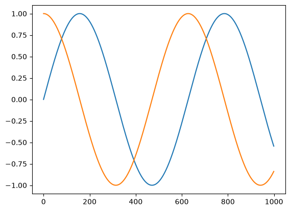
import matplotlib.pyplot as plt

t = jnp.linspace(0, 10, 1000)

plt.plot(jnp.sin(t))
plt.plot(vmap(grad(jnp.sin))(t))

[<matplotlib.lines.Line2D at 0x78e6a29a9d00>]

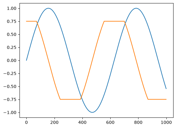
def clip_sin(x):
  x = clip_gradient(-0.75, 0.75, x)
  return jnp.sin(x)

plt.plot(clip_sin(t))
plt.plot(vmap(grad(clip_sin))(t))

[<matplotlib.lines.Line2D at 0x78e6a2a20260>]

Example: Python debugging

Another application that is motivated by development workflow rather than numerics is to set a pdb debugger trace in the backward pass of reverse-mode autodiff.

When trying to track down the source of a nan runtime error, or just examine carefully the cotangent (gradient) values being propagated, it can be useful to insert a debugger at a point in the backward pass that corresponds to a specific point in the primal computation:

import pdb

class Debug(VJPHiPrimitive):
  def __init__(self, x_aval):
    self.in_avals = (x_aval,)
    self.out_aval = x_aval
    self.params = {}
    super().__init__()

  def expand(self, x):
    return x  # acts like identity

  def vjp_fwd(self, nzs_in, x):
    return self(x), x

  def vjp_bwd_retval(self, x, g):
    pdb.set_trace()
    return (g,)

def debug(x):
  return Debug(jax.typeof(x))(x)

def foo(x):
  y = x ** 2
  y = debug(y)  # insert pdb in corresponding backward pass step
  return jnp.sin(y)

jax.grad(foo)(3.)

> <ipython-input-113-b19a2dc1abf7>(12)vjp_bwd_retval()
-> return (g,)
(Pdb) p x
Array(9., dtype=float32)
(Pdb) p g
Array(-0.91113025, dtype=float32)
(Pdb) q

Example: Implicit function differentiation of iterative implementations

This example gets pretty deep in the mathematical weeds!

Another application for custom VJP rules is reverse-mode differentiation of functions that are JAX-transformable (by jit, vmap, …) but not efficiently JAX-differentiable for some reason, perhaps because they involve lax.while_loop. (It’s not possible to produce an XLA HLO program that efficiently computes the reverse-mode derivative of an XLA HLO While loop because that would require a program with unbounded memory use, which isn’t possible to express in XLA HLO, at least without side-effecting interactions through infeed/outfeed.)

For example, consider this fixed_point routine which computes a fixed point by iteratively applying a function in a while_loop:

from jax.lax import while_loop

def fixed_point(f, a, x_guess):
  def cond_fun(carry):
    x_prev, x = carry
    return jnp.abs(x_prev - x) > 1e-6

  def body_fun(carry):
    _, x = carry
    return x, f(a, x)

  _, x_star = while_loop(cond_fun, body_fun, (x_guess, f(a, x_guess)))
  return x_star

This is an iterative procedure for numerically solving the equation \(x = f(a, x)\) for \(x\), by iterating \(x_{t+1} = f(a, x_t)\) until \(x_{t+1}\) is sufficiently close to \(x_t\). The result \(x^*\) depends on the parameters \(a\), and so we can think of there being a function \(a \mapsto x^*(a)\) that is implicitly defined by equation \(x = f(a, x)\).

We can use fixed_point to run iterative procedures to convergence, for example running Newton’s method to calculate square roots while only executing adds, multiplies, and divides:

def newton_sqrt(a):
  update = lambda a, x: 0.5 * (x + a / x)
  return fixed_point(update, a, a)

print(newton_sqrt(2.))

1.4142135

We can vmap or jit the function as well:

print(jit(vmap(newton_sqrt))(jnp.array([1., 2., 3., 4.])))

[1.        1.4142135 1.7320509 2.       ]

We can’t apply reverse-mode automatic differentiation because of the while_loop, but it turns out we wouldn’t want to anyway: instead of differentiating through the implementation of fixed_point and all its iterations, we can exploit the mathematical structure to do something that is much more memory-efficient (and FLOP-efficient in this case, too!). We can instead use the implicit function theorem [Prop A.25 of Bertsekas’s Nonlinear Programming, 2nd ed.], which guarantees (under some conditions) the existence of the mathematical objects we’re about to use. In essence, we linearize at the solution and solve those linear equations iteratively to compute the derivatives we want.

Consider again the equation \(x = f(a, x)\) and the function \(x^*\). We want to evaluate vector-Jacobian products like \(v^\mathsf{T} \mapsto v^\mathsf{T} \partial x^*(a_0)\).

At least in an open neighborhood around the point \(a_0\) at which we want to differentiate, let’s assume that the equation \(x^*(a) = f(a, x^*(a))\) holds for all \(a\). Since the two sides are equal as functions of \(a\), their derivatives must be equal as well, so let’s differentiate both sides:

\(\qquad \partial x^*(a) = \partial_0 f(a, x^*(a)) + \partial_1 f(a, x^*(a)) \partial x^*(a)\).

Setting \(A = \partial_1 f(a_0, x^*(a_0))\) and \(B = \partial_0 f(a_0, x^*(a_0))\), we can write the quantity we’re after more simply as

\(\qquad \partial x^*(a_0) = B + A \partial x^*(a_0)\),

or, by rearranging,

\(\qquad \partial x^*(a_0) = (I - A)^{-1} B\).

That means we can evaluate vector-Jacobian products like

\(\qquad v^\mathsf{T} \partial x^*(a_0) = v^\mathsf{T} (I - A)^{-1} B = w^\mathsf{T} B\),

where \(w^\mathsf{T} = v^\mathsf{T} (I - A)^{-1}\), or equivalently \(w^\mathsf{T} = v^\mathsf{T} + w^\mathsf{T} A\), or equivalently \(w^\mathsf{T}\) is the fixed point of the map \(u^\mathsf{T} \mapsto v^\mathsf{T} + u^\mathsf{T} A\). That last characterization gives us a way to write the VJP for fixed_point in terms of a call to fixed_point! Moreover, after expanding \(A\) and \(B\) back out, we can see we need only to evaluate VJPs of \(f\) at \((a_0, x^*(a_0))\).

Here’s the upshot. The function argument f isn’t differentiated, so it goes in params (functions are hashable), while a and x_guess are ordinary traced inputs:

from functools import partial
from jax import vjp

class FixedPoint(VJPHiPrimitive):
  def __init__(self, a_aval, x_aval, *, f):
    self.in_avals = (a_aval, x_aval)
    self.out_aval = x_aval
    self.params = dict(f=f)
    super().__init__()

  def expand(self, a, x_guess):
    def cond_fun(carry):
      x_prev, x = carry
      return jnp.abs(x_prev - x) > 1e-6

    def body_fun(carry):
      _, x = carry
      return x, self.f(a, x)

    _, x_star = while_loop(cond_fun, body_fun, (x_guess, self.f(a, x_guess)))
    return x_star

  def vjp_fwd(self, nzs_in, a, x_guess):
    x_star = self(a, x_guess)
    return x_star, (a, x_star)

  def vjp_bwd_retval(self, res, x_star_bar):
    a, x_star = res
    _, vjp_a = vjp(lambda a: self.f(a, x_star), a)
    a_bar, = vjp_a(fixed_point(partial(rev_iter, self.f),
                               (a, x_star, x_star_bar),
                               x_star_bar))
    return a_bar, jnp.zeros_like(x_star)

def rev_iter(f, packed, u):
  a, x_star, x_star_bar = packed
  _, vjp_x = vjp(lambda x: f(a, x), x_star)
  return x_star_bar + vjp_x(u)[0]

def fixed_point(f, a, x_guess):
  a_aval = jax.tree.map(jax.typeof, a)
  x_aval = jax.tree.map(jax.typeof, x_guess)
  return FixedPoint(a_aval, x_aval, f=f)(a, x_guess)

print(newton_sqrt(2.))

1.4142135

print(grad(newton_sqrt)(2.))
print(grad(grad(newton_sqrt))(2.))

0.35355338
-0.088388346

We can check our answers by differentiating jnp.sqrt, which uses a totally different implementation:

print(grad(jnp.sqrt)(2.))
print(grad(grad(jnp.sqrt))(2.))

0.35355338
-0.08838835

Notice that the backward rule calls fixed_point again, on the linear problem, and that the parameter a passed there is a pytree of arrays: the in_avals entries can themselves be pytrees of types, as discussed below.

A limitation to this approach is that the argument f can’t close over any values involved in differentiation, since it’s a static parameter of the primitive. That is, you might notice that we kept the parameter a explicit in the argument list of fixed_point. For this use case, consider using the low-level primitive lax.custom_root, which allows for derivatives in closed-over variables with custom root-finding functions.

Basic usage of VJPHiPrimitive

Anatomy of a hijax primitive

A hijax primitive is a subclass of VJPHiPrimitive. Its __init__ must set three attributes before calling super().__init__():

• in_avals, a tuple with one entry per positional argument, giving each argument’s type (each entry can also be a pytree of types);

• out_aval, the output type (also possibly a pytree of types);

• params, a dict of hashable static parameters, which are made available as attributes on the instance (e.g. self.f for params = dict(f=f)). Params are static: they’re baked into the primitive instance, so they can’t be traced values, and dynamic data must instead be an input.

Since the types are fixed at construction time, the usual idiom is a wrapper function that builds the primitive instance from the types of the arguments, using jax.typeof, and immediately applies it:

class Square(VJPHiPrimitive):
  def __init__(self, x_aval):
    self.in_avals = (x_aval,)
    self.out_aval = x_aval
    self.params = {}
    super().__init__()

  def expand(self, x):
    return x * x

def square(x):
  return Square(jax.typeof(x))(x)

print(square(3.))

9.0

The instance is callable, and calling it is what binds the primitive: in an eager context it evaluates, and under a jit trace it records itself into the jaxpr as a single equation. The types of the actual arguments are checked against in_avals.

The only required method is expand, which gives the implementation as a JAX-traceable Python function of the (non-static) arguments. Everything else is optional, and is only needed if you use the corresponding transformation:

method(s)	transformation
expand	evaluation and lowering (jit)
vjp_fwd and vjp_bwd_retval (or vjp_bwd)	reverse-mode autodiff (grad, vjp)
jvp	forward-mode autodiff (jvp)
lin and linearized	jax.linearize
batch_dim_rule (or batch)	vmap
transpose	transposition, for primitives linear in some inputs

If you apply a transformation without having defined the corresponding method, you get a NotImplementedError telling you what to implement. For a primitive with a jvp rule, the reverse-mode and linearize methods can also be derived automatically — see the helpers below.

Custom VJPs with vjp_fwd and vjp_bwd_retval

The pair vjp_fwd/vjp_bwd_retval works just like the f_fwd/f_bwd pair of jax.custom_vjp, in Haskell-like type signatures:

vjp_fwd :: (NonZeros, a) -> (b, c)
vjp_bwd_retval :: (c, CT b) -> CT a

The function vjp_fwd describes the forward pass: it takes the primal inputs and returns a pair of the primal output and any “residual” data to be stored for use by the backward pass. (Its extra first argument nzs_in is a tuple of booleans indicating which inputs are being differentiated; you can ignore it, or use it to avoid saving residuals that won’t be needed.) The primal output should usually be computed by calling self(...), i.e. by binding the primitive itself; that way the custom rules also apply under higher-order differentiation.

The function vjp_bwd_retval describes the backward pass: it takes the residuals and the cotangent of the output, and returns a tuple of cotangents with one entry per primal input.

class Mul(VJPHiPrimitive):
  def __init__(self, x_aval, y_aval):
    self.in_avals = (x_aval, y_aval)
    self.out_aval = x_aval
    self.params = {}
    super().__init__()

  def expand(self, x, y):
    return x * y

  def vjp_fwd(self, nzs_in, x, y):
    return self(x, y), (x, y)

  def vjp_bwd_retval(self, res, g):
    x, y = res
    return (g * y, x * g)

def mul(x, y):
  return Mul(jax.typeof(x), jax.typeof(y))(x, y)

print(grad(mul)(2., 3.))
print(grad(mul, 1)(2., 3.))

3.0
2.0

Custom JVPs with jvp

The jvp method defines forward-mode differentiation. It takes a tuple of primal inputs and a tuple of tangent inputs, and returns a pair of the primal output and the tangent output. (The input tangents can be symbolic zeros in some cases; see the symbolic zeros section below.)

class Sin(VJPHiPrimitive):
  def __init__(self, x_aval):
    self.in_avals = (x_aval,)
    self.out_aval = x_aval
    self.params = {}
    super().__init__()

  def expand(self, x):
    return jnp.sin(x)

  def jvp(self, primals, tangents):
    (x,), (x_dot,) = primals, tangents
    return self(x), jnp.cos(x) * x_dot

def sin(x):
  return Sin(jax.typeof(x))(x)

y, y_dot = jvp(sin, (3.,), (1.,))
print(y)
print(y_dot)

0.14112
-0.9899925

One difference from jax.custom_jvp: by default, JAX does not automatically derive reverse-mode differentiation from a hijax primitive’s jvp rule, so applying grad to sin as defined above raises a NotImplementedError asking for vjp_fwd. You can define both sets of rules on the same primitive (as in the TL;DR example above); unlike with jax.custom_jvp and jax.custom_vjp, you never have to choose between them.

But you can also opt into jax.custom_jvp-style behavior, where everything is derived from the JVP rule, by assigning helper functions as class attributes. The helpers come in pairs: lin = linearize_from_jvp together with linearized = apply_derived_linearization derives linearization support by partially evaluating jvp, and vjp_fwd = vjp_fwd_from_jvp together with vjp_bwd_retval = transpose_jvp derives reverse mode by storing the primal inputs and then linearizing and transposing jvp on the backward pass:

from jax.experimental.hijax import (
    linearize_from_jvp, apply_derived_linearization,
    vjp_fwd_from_jvp, transpose_jvp)

class SinAD(Sin):
  lin = linearize_from_jvp
  linearized = apply_derived_linearization
  vjp_fwd = vjp_fwd_from_jvp
  vjp_bwd_retval = transpose_jvp

def sin(x):
  return SinAD(jax.typeof(x))(x)

print(grad(sin)(3.))
y, sin_lin = jax.linearize(sin, 3.)
print(sin_lin(1.))
print(grad(grad(sin))(3.))

-0.9899925
-0.9899925
-0.14112

As with jax.custom_jvp, for the derived transposition to work, the JVP rule’s output tangents must be linear as a function of the input tangents.

A second pair, vjp_fwd = vjp_fwd_from_lin with vjp_bwd_retval = transpose_linearized, instead derives reverse mode from the lin/linearized rules (whether handwritten or themselves derived from jvp): it stores the linearization’s residuals rather than the primal inputs, and transposes linearized on the backward pass. And jvp = jvp_from_lin goes the other way, deriving forward mode from handwritten lin/linearized rules. (Deriving in a circle, with jvp = jvp_from_lin and lin = linearize_from_jvp on the same primitive, is an error.)

Both kinds of rules are also what make higher-order differentiation work: grad-of-grad composes the VJP rules, while e.g. jax.hessian, which is forward-over-reverse, needs the jvp rule as well. As with jax.custom_jvp and jax.custom_vjp, a rule applies at higher orders of differentiation only if it computes its primal output by binding the primitive itself, i.e. by calling self(...) rather than inlining the implementation. (This represents a kind of fundamental tradeoff, where we can’t make use of intermediate values from the evaluation of expand in our rule and also have the rule apply in all orders of higher-order differentiation.)

Hijax primitives in jaxprs

Because a hijax primitive is a real primitive, it appears as a single equation in jaxprs:

make_jaxpr(mul)(2., 3.)

{ lambda ; a:f32[] b:f32[]. let
    c:f32[] = call_hi_primitive[_prim=Mul[{}]] a b
  in (c,) }

That’s true under jit too. It’s only at lowering time that expand is traced and inlined. In an eager context, each call to the primitive calls expand again (so, like any JAX function, it’s best to keep expand free of side effects, though harmless ones like print can be instructive):

class Noisy(VJPHiPrimitive):
  def __init__(self, x_aval):
    self.in_avals = (x_aval,)
    self.out_aval = x_aval
    self.params = {}
    super().__init__()

  def expand(self, x):
    print('called expand!')
    return jnp.sin(x)

def noisy(x):
  return Noisy(jax.typeof(x))(x)

print(noisy(3.))

called expand!
0.14112

print(jit(noisy)(3.))
print(jit(noisy)(3.))  # tracing is cached: no more 'called expand!'

called expand!
0.14112
0.14112

You can also use Python control flow in expand and in the derivative rules, as long as the primitive is used eagerly (outside of jit), since the rules then see concrete values:

class G(VJPHiPrimitive):
  def __init__(self, x_aval):
    self.in_avals = (x_aval,)
    self.out_aval = x_aval
    self.params = {}
    super().__init__()

  def expand(self, x):
    if x > 0:
      return jnp.sin(x)
    else:
      return jnp.cos(x)

  def vjp_fwd(self, nzs_in, x):
    return self(x), x

  def vjp_bwd_retval(self, x, g):
    if x > 0:
      return (2 * g,)
    else:
      return (3 * g,)

def g(x):
  return G(jax.typeof(x))(x)

print(grad(g)(1.))
print(grad(g)(-1.))

2.0
3.0

vmap with batch_dim_rule

For vmap support, the easiest option is to define batch_dim_rule, which takes axis metadata and the batch dimension of each argument (None for unbatched arguments) and just returns the batch dimension of the output. Given that data movement answer, JAX derives the batched computation automatically by vmap-ing the primitive’s other rules:

class MulV(Mul):
  def batch_dim_rule(self, axis_data, in_dims):
    x_dim, y_dim = in_dims
    return y_dim if x_dim is None else x_dim

def mul(x, y):
  return MulV(jax.typeof(x), jax.typeof(y))(x, y)

x = jnp.arange(3.)
y = jnp.arange(3.) + 1.
print(vmap(mul)(x, y))
print(vmap(mul, in_axes=(0, None))(x, 2.))
print(vmap(grad(mul))(x, y))

[0. 2. 6.]
[0. 2. 4.]
[1. 2. 3.]

(For full control over the batched computation itself, you can instead override the batch method.)

More features and details

Working with list / tuple / dict containers (and other pytrees)

The entries of in_avals, and out_aval itself, can be pytrees of types, so arguments and outputs can be pytrees of arrays. Here’s a contrived example:

from collections import namedtuple
Point = namedtuple("Point", ["x", "y"])

from jax.experimental.hijax import Zero, instantiate_zeros

class FPt(VJPHiPrimitive):
  def __init__(self, pt_aval):
    self.in_avals = (pt_aval,)
    self.out_aval = {'a': pt_aval.x, 'b': (pt_aval.x, pt_aval.y)}
    self.params = {}
    super().__init__()

  def expand(self, pt):
    return {'a': pt.x ** 2, 'b': (jnp.sin(pt.x), jnp.cos(pt.y))}

  def vjp_fwd(self, nzs_in, pt):
    return self(pt), pt

  def vjp_bwd_retval(self, pt, g):
    g = jax.tree.map(instantiate_zeros, g,
                     is_leaf=lambda x: isinstance(x, Zero))
    a_bar, (b0_bar, b1_bar) = g['a'], g['b']
    x_bar = 2 * pt.x * a_bar + jnp.cos(pt.x) * b0_bar
    y_bar = -jnp.sin(pt.y) * b1_bar
    return (Point(x_bar, y_bar),)

def f(pt):
  return FPt(jax.tree.map(jax.typeof, pt))(pt)

def fun(pt):
  dct = f(pt)
  return dct['a'] + dct['b'][0]

pt = Point(1., 2.)
print(f(pt))
print(grad(fun)(pt))

{'a': 1.0, 'b': (Array(0.84147096, dtype=float32, weak_type=True), Array(-0.41614684, dtype=float32, weak_type=True))}
Point(x=Array(2.5403023, dtype=float32, weak_type=True), y=Array(-0., dtype=float32, weak_type=True))

Symbolic zeros

The example above snuck in a new detail: the cotangents passed to the backward rule can contain symbolic zeros. When part of the primitive’s output doesn’t affect the value being differentiated (here fun doesn’t use dct['b'][1]), the corresponding cotangent is not an array of zeros but an instance of the special Zero class, which records only the type. That’s in contrast to jax.custom_vjp, where symbolic zeros are opt-in via symbolic_zeros=True.

Symbolic zeros let a rule avoid doing work (or avoid errors, for non-differentiable outputs like integer values). If you don’t want to handle them, instantiate them into actual zero arrays with instantiate_zeros, as above.

On the input side, the nzs_in argument to vjp_fwd reports symbolically which inputs are being differentiated: it’s a tuple of booleans, one per input, where False means that input’s tangent is symbolically zero, so no cotangent for it will be used. A rule can use that to avoid saving unneeded residuals:

class Mul2(VJPHiPrimitive):
  def __init__(self, x_aval, y_aval):
    self.in_avals = (x_aval, y_aval)
    self.out_aval = x_aval
    self.params = {}
    super().__init__()

  def expand(self, x, y):
    return x * y

  def vjp_fwd(self, nzs_in, x, y):
    x_nz, y_nz = nzs_in
    return self(x, y), (x if y_nz else None, y if x_nz else None)

  def vjp_bwd_retval(self, res, g):
    x, y = res
    return (g * y if y is not None else None,
            x * g if x is not None else None)

def mul2(x, y):
  return Mul2(jax.typeof(x), jax.typeof(y))(x, y)

print(grad(mul2, 0)(2., 3.))  # nzs_in == (True, False), saves only y
print(grad(mul2, 1)(2., 3.))  # nzs_in == (False, True), saves only x

3.0
2.0

Notice that the backward rule can return None for an input whose cotangent isn’t needed.

Symbolic zeros appear on the forward-mode side too: the tangents passed to a jvp rule can be Zeros, for example when a primitive is applied to a mix of differentiated inputs and constants. That’s true whether the rule is invoked directly by jax.jvp or partially evaluated by linearize_from_jvp. As with cotangents, a rule can handle them explicitly to exploit the sparsity, or clean them up with instantiate_zeros.

In-place cotangent accumulation with vjp_bwd

Instead of vjp_bwd_retval, which returns the input cotangents as values, a backward rule can be written as vjp_bwd, which receives one accumulator per primal input and adds each cotangent contribution in-place by calling .accum(...):

class Mul3(VJPHiPrimitive):
  def __init__(self, x_aval, y_aval):
    self.in_avals = (x_aval, y_aval)
    self.out_aval = x_aval
    self.params = {}
    super().__init__()

  def expand(self, x, y):
    return x * y

  def vjp_fwd(self, nzs_in, x, y):
    return self(x, y), (x, y)

  def vjp_bwd(self, res, g, x_acc, y_acc):
    x, y = res
    x_acc.accum(g * y)
    y_acc.accum(x * g)

def mul3(x, y):
  return Mul3(jax.typeof(x), jax.typeof(y))(x, y)

print(grad(mul3)(2., 3.))

3.0

For inputs that aren’t being differentiated, the accumulator is a NullAccum whose accum is a no-op, so it’s safe to accumulate unconditionally. The accumulator form can save memory when gradients are accumulated across many contributions. Define either vjp_bwd or vjp_bwd_retval, not both.

Custom linearization with lin and linearized

jax.linearize doesn’t use the jvp or VJP rules; it has its own pair of methods. The lin method is like vjp_fwd: it takes nzs_in and the primal inputs, and returns the primal output paired with residuals. The linearized method is the linear map itself: it takes the residuals and the input tangents, and returns the output tangents:

class Sin2(Sin):
  def lin(self, nzs_in, x):
    return self(x), jnp.cos(x)

  def linearized(self, cos_x, x_dot):
    return cos_x * x_dot

def sin2(x):
  return Sin2(jax.typeof(x))(x)

y, f_lin = jax.linearize(sin2, 3.)
print(y)
print(f_lin(1.))

0.14112
-0.9899925

(If you don’t need to control the linearization itself, recall from above that a primitive with a jvp rule can just set lin = linearize_from_jvp and linearized = apply_derived_linearization.)

What we haven’t covered

Custom derivatives are only part of the hijax story. Hijax primitives can also:

• introduce new types beyond arrays, by subclassing HiType (immutable) or MutableHiType and registering them with register_hitype, with the primitive’s in_avals/out_aval mentioning the new types;

• define a transpose rule, for primitives that are linear in some inputs;

• customize rematerialization via a remat method, and dead code elimination via a dce method.

Those deserve documents of their own. In the meantime, tests/hijax_test.py is a good source of worked examples.